How to do the IGNOU MGGL 003 Practical yourself, session by session
The IGNOU MGGL 003 Practical works best as a running lab diary in QGIS: each of the 22 exercises gets one entry, written in its own session, that names the data, the settings and the output, so the record and the viva rest on work you can repeat on demand.
The method in one box
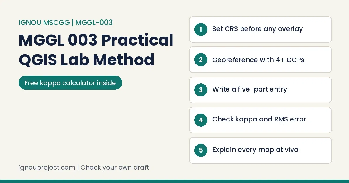
To complete the IGNOU MGGL 003 Practical, install QGIS before Day 1, work two exercises a day from Day 1 to Day 11, write a five-part entry for each before you leave the lab, check every output against its source, and use Day 13 to assemble a record you can explain at the Day 14 viva-voce.
MGGL-003 Geospatial Analysis is the 4-credit lab course of MSCGG Semester III, planned as 26 laboratory sessions over 14 days with a counsellor guiding the exercises; its GIS theory sits in MGG-011. This guide covers the doing: setup, the entry, three worked exercises, mistakes and a final self-check.
What to set up before Day 1 of the lab
Most of the IGNOU MGGL 003 Practical depends on things you can arrange at home in an evening, and because the software is open source you can rehearse any exercise after the session ends.
- QGIS on your own computer. Exercise 2 walks through installation. The course book fixes no version (Exercise 10 was made on 3.28; references cite the 3.34 guide), so match the release on your lab machines.
- A GEE account. The Google Earth Engine plugin in Exercise 5 (Day 3) needs one.
- Your own locality. Exercise 5 asks you to repeat its tasks on a neighbourhood, campus or place you know, and Exercise 9 asks for garbage disposal sites in your area. Pick one area now and keep it.
A five-part entry for every exercise in the IGNOU MGGL 003 Practical
Every exercise in the IGNOU MGGL 003 Practical ends with practical questions, and your entry should answer them rather than narrate clicks.
Five parts of every entry
- Aim, taken from the wording of the practical question (for Exercise 17: compare the optimum path with the straight-line distance).
- Data and CRS: file names, where the data came from (given file, OpenStreetMap, SRTM or ALOS, Sentinel-2), the coordinate reference system with its EPSG code, and the area covered.
- Method: the menu path or Processing tool, the plugin, and every parameter you set, such as the transformation type or a threshold value.
- Output: the map, table or chart, its file name, and for a map the layout elements it carries.
- Reading: what the output shows in two or three sentences, one number taken from it, and the likely sources of error.
Across practical courses we see entries that only describe actions, such as loading a layer and running a tool, repeated page after page; an evaluator looks for each step to be tied to the method or idea behind it. In MGGL-003 the practical questions name that idea for you, for example the transformation method and the RMS error in Exercise 3.
A log written in one sitting at the end gives itself away: sentences repeat, dates fall on days with no class, and the last entry reads no more skilled than the first. The MGGL-003 course book sets two sessions on each of its 14 days.
Worked example: georeferencing in QGIS for Exercise 3
Georeferencing appeared in all three Set-I papers published so far, which makes Exercise 3 the best place in the IGNOU MGGL 003 Practical to rehearse the five-part entry. The steps follow the course book’s first method, assigning coordinates to a scanned sheet.
Exercise 3 georeferencing, worked
- Open Raster, then Georeferencer, and load the scanned map from your exercise folder.
- Choose Add Point and click the top-left intersection of latitude and longitude, with the crosshair exactly on the crossing. Type the printed values in the dialog.
- Repeat at the other three corners until the GCP table lists four points. For raster-to-raster work, choose From Map Canvas and click the same feature on a georeferenced image.
- Open Settings, then Transformation Settings. Choose the transformation the question asks for (Linear, Helmert or Polynomial), the target CRS and the output file name.
- Click Start Georeferencing, open the result, and overlay a georeferenced satellite base (the question names Google Satellite or Bing Aerial) to look for features that drift.
One detail matters here. In QGIS a first-order polynomial needs at least three GCPs, a second-order six and a third-order ten. With exactly three points the fit has no spare point, every residual reads zero and the RMS error means nothing; four or more well-spread points give an error you can report.
Your entry then reads, with your own values in the brackets: Aim: georeference the given scanned sheet. Data: scanned map, four corner GCPs from the printed graticule, target CRS [EPSG code]. Method: Georeferencer, [transformation], output GeoTIFF. Output: georeferenced raster, RMS error [value] from the GCP table. Reading: alignment against the satellite base, largest residual at [corner], likely cause [scan distortion, paper shrinkage or a misplaced click].
Accuracy assessment for Exercise 13, with a kappa coefficient calculator
Exercise 13 wants at least five land use and land cover classes, classified with Maximum Likelihood or Random Forest in SCP, then checked against validation points. The course book’s Table 13.3 puts classified classes in rows and validation classes in columns for four classes (Water, Built-up, Vegetation, Barren/soil); the illustration adds Cropland to reach five.
Illustrative five-class error matrix
| Classified (rows) / Validation (columns) | Water | Built-up | Vegetation | Barren/soil | Cropland | Row total |
|---|---|---|---|---|---|---|
| Water | 44 | 1 | 2 | 0 | 1 | 48 |
| Built-up | 1 | 37 | 2 | 6 | 4 | 50 |
| Vegetation | 2 | 2 | 48 | 1 | 7 | 60 |
| Barren/soil | 0 | 5 | 1 | 30 | 4 | 40 |
| Cropland | 1 | 3 | 6 | 3 | 39 | 52 |
| Column total | 48 | 48 | 59 | 40 | 55 | 250 |
The counts are invented for practice and are not from the course book; your own SCP accuracy table replaces them.
Working. Overall accuracy is the diagonal over the total: 198 / 250 = 79.2 percent. Chance agreement is the sum of row total times column total over the total squared: 12,704 / 62,500 = 0.2033. Kappa = (0.792 – 0.2033) / (1 – 0.2033) = 0.739. User’s accuracy reads along a row (Built-up 37 / 50 = 74.0 percent); producer’s accuracy reads down a column (Built-up 37 / 48 = 77.1 percent). Name the weakest class and why: here Cropland, 70.9 percent producer’s accuracy, confused with Vegetation.
Kappa and accuracy calculator
Enter your own counts (rows classified, columns validation) and press Calculate.
Result: overall 79.2 percent, kappa 0.739 for the preloaded matrix.
In lab records across courses, the weak ones share a look: tables without totals, workings that stop before the answer, maps with no labels, and nothing said about error. In MGGL-003, the fifth practical question of Exercise 13 names all four accuracy figures, kappa included, as the things to report.
Writing up RUSLE in QGIS for Exercise 12
In the IGNOU MGGL 003 Practical, Exercise 12 estimates annual soil loss as A = R x K x LS x C x P, in tons per hectare per year, building each factor as a raster first. Record each layer's source.
- R, rainfall erosivity: a constant or interpolated raster; the book's example for a constant of 500 is the expression "DEM@1" * 0 + 500.
- K, soil erodibility: values assigned by soil texture class on the soil map, then Rasterize (vector to raster).
- LS, slope length and steepness: from the Exercise 11 slope raster, through the LS Factor plugin or the book's approximation using flow accumulation and cell size.
- C, cover management: from land use, for example Forest 0.001, Grassland 0.01, Cropland 0.5.
- P, conservation practice: Contour farming 0.5, Terracing 0.1, No practice 1.
- Multiply in Raster Calculator: "R.tif" * "K.tif" * "LS.tif" * "C.tif" * "P.tif".
RUSLE one-cell spot check
Read one pixel in all five factor rasters with Identify Features. Suppose R is 500 (the book's constant), K is 0.3 and LS is 2.0 (both illustrative), C is 0.5 for cropland and P is 0.5 for contour farming: 500 x 0.3 x 2.0 x 0.5 x 0.5 = 75 tons per hectare per year. A different value in the output means a layer has wrong units, a shifted extent or a NoData cell.
For the high-risk zones the question asks for, reclassify the soil loss raster, show your class breaks in the legend, and tie each conservation measure to a factor: terracing changes P, cover crops change C. The book points back to Unit 9 and Exercises 20 and 21 of MGGL-001, which our first-semester cartography guide also works through.
With computer practicals of every kind, a common fault is an output the written command could not have made, or a command printed with nothing to show for it. In MGGL-003, Exercise 12 ends with a single Raster Calculator line in which five factor rasters are multiplied to give soil loss.
Seven mistakes in the IGNOU MGGL 003 Practical and how to fix them
Each comes from a step the course book or a published paper makes explicit.
- Measuring distance or area in degrees. Fix: reproject first; the December 2025 paper asked for geographic coordinates to UTM WGS84 before measuring.
- Bunching GCPs in one corner. Fix: spread at least four well-distributed points, as Exercise 3 asks, and redo any with a large residual.
- Validating with the training polygons. Fix: digitise a separate reality file; the course book calls it an independent reference dataset.
- Reporting overall accuracy alone. Fix: add user's and producer's accuracy for every class and the kappa coefficient.
- Delineating a watershed on a raw DEM. Fix: run Fill Sinks (Wang and Liu) first; Exercise 19 builds flow direction and flow accumulation on the filled DEM.
- Printing a layout with parts missing. Fix: title, scale, north arrow, grid lines and legend, as the June 2026 paper listed; Exercise 10 says study centre printers are generally A4 or A3.
- Practising only on given data. Fix: the June 2026 paper asked for your own area on OpenStreetMap, your examination centre on it, and polygons within 500 m of it, so rehearse on your locality.
Another mistake is to treat the viva as a formality. It usually counts for a good deal, and a tidy file earns little when its owner cannot state the aim, the method or what the result shows. MGGL-003 holds its viva-voce in Session 2 of Day 14.
Finished practical files are passed around online, and some are handed in with only a new name and enrolment number; several identical files from one centre are noticed quickly, and the viva shows who cannot explain the work. In MGGL-003, the second practical question of Exercise 9 asks you to locate garbage disposal sites in your own area.
Day 14: the examination drill and MGGL 003 viva questions
The last day of the IGNOU MGGL 003 Practical holds the examination in Session 1 and the viva-voce in Session 2. Each published Set-I paper runs 3 hours for 50 marks, any five of seven questions at 10 marks each: 36 minutes a question. Most questions pair a short written part with a QGIS task, so rehearse both halves together, timing five questions from one paper. The examination fee (Rs 300 for a practical course of up to 4 credits) goes with your TEE form.
MGGL 003 viva questions to practise
The course book prints no viva list; these are built from the exercises.
- Which CRS did you use to measure distance and area, and why not degrees?
- How many GCPs did you place, which transformation did you choose, and what was the RMS error?
- In your Exercise 13 matrix, which class had the lowest producer's accuracy, and what does kappa add to overall accuracy?
- Why must the DEM be filled before flow direction is computed?
- Where did each RUSLE factor in your map come from, and which one varies most across your area?
- Which project area from Exercises 23 to 25 did you pick, and why that place?
Self-check before you hand in the record
Records for the IGNOU MGGL 003 Practical are prepared in the second session of Day 13; run this list a day earlier so there is time to fix what it finds.
Record audit, eleven points
Title pages often carry a slip: an enrolment number off by a digit, the wrong programme, or a mistaken study centre code. Since the MGGL-003 course book gives no cover layout, take the first-page fields from your counsellor.
A counsellor signature that nobody collected tends to surface only on the day of hand-in. The course book for MGGL-003 describes no signature page, so follow what your own counsellor asks for.
Send your own MGGL-003 write-up for a check
If an entry, the Exercise 3 alignment report or the Exercise 13 accuracy write-up reads thin to you, send your own file; we mark gaps against the practical questions and return comments. We do not make your maps or write your entries: you remain the author, IGNOU's evaluator decides the result, and no marks are promised. You can send your file for a check through this page or on WhatsApp at +91 93546 37830. For the MGGP-001 synopsis that Days 12 and 13 begin, the services and charges page prints synopsis correction at Rs 1,000, and our MGGP-001 project guide explains the project itself.
Across lab courses, the record is where we watch the most marks drain away, and it is the part most easily put right. In MGGL-003, preparation of practical records follows Exercise 25 on Day 13.
Short answers on the IGNOU MGGL 003 Practical
Can I practise the IGNOU MGGL 003 Practical at home?
Yes. QGIS and its plugins are free, and the portals in Exercises 21 and 22 (Google Earth, Bhuvan, VEDAS, India-WRIS) are online. The course book still asks you to complete the 26 laboratory sessions, so home practice adds to the lab days rather than replacing them.
Does the course book give a fixed record format?
No. It sets no page order, cover layout or marks split, so the content follows each exercise's practical questions; ask your counsellor whether maps go in printed or as files.
Can someone else prepare my MGGL-003 record?
No. It must come from your own sessions, and the viva tests whether you can explain it. We only check a draft you have written.
Finishing the IGNOU MGGL 003 Practical on work you can explain
Work the IGNOU MGGL 003 Practical in order, write each entry in its session, test your numbers with the two tools above, and walk into Day 14 with maps of a place you know. Printed reference material for this course is on our publication site.
The learners who finish well tend to begin early, check the rules at the centre where they are enrolled, date an entry for each session, gather signatures along the way, and know each page well enough to talk through it unaided. MGGL-003 gives you 26 laboratory sessions in which to build that habit.
Official documents behind this guide
- MGGL-003 Geospatial Analysis course book, School of Sciences, IGNOU, February 2026 print (eGyanKosh, MSCGG Semester III)
- IGNOU Common Prospectus July 2026: section 3.54 (MSCGG) and the practical examination fee
- June 2025 Set-I paper of MGGL-003
- December 2025 Set-I paper of MGGL-003
- June 2026 Set-I paper of MGGL-003
Documents read in November 2026: the MGGL-003 course book (guidelines, day plan, all 22 exercises), the July 2026 Common Prospectus (MSCGG section and fee rules) and the three published Set-I papers. Drafting was AI-assisted, every rule was checked against the sources listed, and BK Sahni publishes this guide under his editorial responsibility.
ignouproject.com is not affiliated with, authorised by or endorsed by IGNOU. We check and correct the learner's own work; you remain the author of your record and project.

BK Sahni iD 0009-0005-8092-459X
Founder, Shri Chakradhar Publication Pvt. Ltd. & ignouproject.com — helping IGNOU distance-learning students since 2010 (5,00,000+ students supported across MBA, MCom, MA & more). Author of IGNOU exam guides, solved assignments & project reference books.
Disclosure: Shri Chakradhar Publication Pvt. Ltd. and ignouproject.com are independent third-party study-help services — not the official IGNOU website. Always verify final dates and rules on ignou.ac.in.